Making AI Decisions Transparent

---

What is Model Explanability

Artificial intelligence is becoming a key player in industries ranging from finance to healthcare. But as AI models grow more complex, their decisions often feel like a "black box"—we see the outcomes, but we don’t always understand how they were reached. This is where model explanability comes in.

Model explanability refers to the ability to interpret and understand how an AI model makes predictions or decisions. Some models, like simple decision trees, are naturally interpretable, while deep learning models and large language models (LLMs) require additional techniques to uncover their reasoning. The goal is to bring transparency, making AI more trustworthy and responsible.

Why is Model Explanability so Important

Explanability is not just a nice-to-have—it’s essential for ensuring AI is ethical, reliable, and aligned with human values. A few scenarios definitely requires you leverage the explanability to achieve your expected goal:

• Trust building: For businesses and consumers to adopt the decision making by AI. Explanability fosters the confidence so trust towards AI will be built and they won’t feel strong hesitate to adopt it
• Bias&Fairness Correction: AI model will response and generate output affected by the data is was trained on. So explanability comes to rescue and help correct these issues by pinpointing where the problems are
• Regulation Compliance: Laws like AI Act, GDPR and ISO will require AI Models to provide explanation for their decision(output/response), especially in high-risk application. This is obligation and the businesses are mandatory to make these kind of proofs at hand.
• Performance Improvement: Explanability help engineer understand how models make prediction and fine tune it to achieve better accuracy and precision
• Being Responsible: Ethical AI development relies on transparency, preventing harmful or discriminatory decisions from going unchecked

Real-World Applications of Model Explanability

Now, we take a brief of some real word application that AI Model explanability help address the real world problems.

Finance: Understanding Credit Decisions

Financial institutions increasingly use AI models to assess loan applications, set credit limits, and determine interest rates. However, when an applicant is denied a loan or offered unfavorable terms, they deserve to understand why. A lack of transparency can erode trust and raise concerns about fairness and compliance with financial regulations.

Explanability techniques, such as SHAP (Shapley Additive Explanations), help demystify complex credit scoring models by identifying the most influential factors behind a decision. For instance, if a customer’s loan application is rejected, SHAP values can reveal whether the primary reasons were a low credit score, high debt-to-income ratio, or insufficient credit history.

By making AI-driven credit decisions more transparent, financial institutions can improve customer trust, comply with regulations like the Equal Credit Opportunity Act (ECOA), and proactively address potential biases in their lending models.

Healthcare: AI-Assisted Diagnosis

AI is playing a growing role in medical diagnostics, helping detect diseases, recommend treatments, and assess patient risk factors. However, healthcare professionals and patients must understand the rationale behind AI-driven predictions to ensure trust, accountability, and informed decision-making.

Explanability tools, such as LIME (Local Interpretable Model-Agnostic Explanations), provide crucial insights by highlighting which medical indicators contributed most to a given diagnosis. For example, if an AI model predicts that a patient has a high likelihood of developing lung cancer, LIME can reveal whether the model based its prediction on factors such as tumor size, genetic predisposition, or smoking history.

Transparent AI explanations allow doctors to validate AI-driven diagnoses, improve patient-doctor communication, and ensure AI models align with medical best practices and ethical standards.

Legal & Compliance: Ensuring Fairness

Regulatory agencies and businesses are increasingly leveraging AI to conduct audits, enforce compliance, and detect fraudulent activities. However, for AI-driven legal and compliance decisions to be trusted, they must be explainable and free from hidden biases.

For example, AI models are commonly used in hiring decisions to filter candidates based on experience, skills, and qualifications. If a candidate is rejected, explainability techniques can reveal which factors had the greatest impact and whether any unintended biases influenced the decision. This is essential for ensuring compliance with employment laws such as the Equal Employment Opportunity Commission (EEOC) guidelines and preventing discrimination in hiring.

Similarly, in the insurance industry, AI-driven underwriting models assess risk and determine policy pricing. Explainable AI models ensure that decisions are based on relevant risk factors rather than discriminatory attributes, fostering transparency and fairness.

Autonomous Systems: Self-Driving Cars

Self-driving vehicles depend on AI to process real-time sensor data, detect obstacles, and make split-second decisions. However, when unexpected behaviors occur—such as sudden braking or failing to recognize an object—it is crucial to understand why the AI acted as it did.

Explanability techniques analyze the decision pathways of autonomous systems to clarify why an AI model made a particular choice. For example, if a self-driving car unexpectedly stops in the middle of a highway, explanability methods such as saliency maps can reveal whether the AI detected a potential hazard, misinterpreted road signs, or encountered an ambiguous scenario.

By improving transparency in AI-driven decision-making, automakers, regulators, and the public can ensure autonomous systems operate safely, reduce risks, and establish clear accountability in the event of accidents.

How Do We Evaluate Model Explanability

The two most frequently used metrics are: SHAP(Shapley Additive Explanation) and LIME (Local Interpretable Model-Agnostic Explanations). We will demonstrate both cases with simple codes. But before we cut to the codes, allow me illustrate what happens underneath with the plain English as simplified as I can.

What is SHAP

SHAP is based on game theory and assigns each feature an importance value for a particular prediction. It calculates contributions using Shapley values, which represent the average marginal contribution of a feature across all possible feature combinations.

Mathematically, for a prediction function , the Shapley value for a feature is computed as:

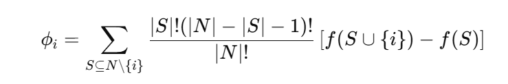
where:

• f is the set of all features,
• S is a subset of features not including feature i ,
• f(S) is the model's prediction for the subsets S ,
• |S| is the number of features in subsets S,
• |N| is the total number of features

Let us go through the main steps of the SHAP computation.

Step 1 Train a model to predict the output

Let's consider a simple example with three features: F={A,B,C} . Assume a model trained with data is :

$$F=β_0+β_1A+β_2B+β_3C$$

Step 2 Consider All Possible Feature Subsets

We will calculate the SHAP value for feature A as illustration. Given this pretext, we list down all the subsets(all excluding A):

• S={}
• S={B}
• S={C}
• S={B,C}

Step 3 Compute marginal contributions for Each Feature subsets

For each Sub set, we define the prediction as these:

• f({}) =10
• f({B}) =12
• f({C}) =14
• f({B,C}) =20
• f({A}) =25
• f({A,B}) =30
• f({A,C}) =40
• f({A,B,C}) =50 hense we will have a table like below

subsets	Marginal contributions	Marginal Contribution Values	Compute Weighting Factors:
S={}	f({A})−f({})	18-10=8	$\cfrac{0!(3-0-1)!}{3!}=\cfrac{1*2}{6}=\cfrac{1}{3}$
S={B}	f({A,B})−f({B})	30-12=18	$\cfrac{1!(3-1-1)!}{3!}=\cfrac{1*1}{6}=\cfrac{1}{6}$
S={C}	f({A,C})−f({C})	40-14=16	$\cfrac{1!(3-1-1)!}{3!}=\cfrac{1*1}{6}=\cfrac{1}{6}$
S={B,C}	f({A,B,C})−f({B,C})	50-20=30	$\cfrac{2!(3-2-1)!}{3!}=\cfrac{2*1}{6}=\cfrac{1}{3}$

Wait! How are these marginal contribution values coming from?

f{()} =10 provide baseline value while no features are used. Given our model formula: F=β0+β1A+β2B+B3C,

• f({}) =$β_0$=10 when no features are used
• f{{B}) =$β_0+β_2B$=12 when only feature B is used

The rest will follow the suite. However, if our model is decision tree or deep network, the subset prediction will vary to a slight degree.

• The decision tree requires all features participate in subtree splitting, so the baseline prediction for decision tree is the average value of the target variable in the training data (for regression) or the most frequent class (for classification).
• And for the deep learning network, NN for instance, the baseline prediction is determined by the bias terms in the output layer when all input features are set to zero (or their default values). In another words, the last layer(output layer) is doing the same way as linear regression will be doing for base predictions.

Step 4 Compute SHAP value for Each Feature subsets

Let us calculate the SHAP value for feature A: Pardon me for taking a second off from doing the calculation and you shall be savvy enough to solve the equation given all the values in the above

Talk is cheap and show me the codes

we will get the customer churn dataset from Kaggle and feed into a xgboost model, then construct a SHAP Explainer class, followed charts to visualize the importance of each features.

#!pip install shap
#!pip install xgboost
#!pip install sklearn
import shap
import xgboost
import pandas as pd
from sklearn.model_selection import train_test_split
shap.initjs()

#download test data from https://www.kaggle.com/datasets/royjafari/customer-churn?resource=download
#And place it somewhere in the local
#Please change in accordance to your local path
dataframe = pd.read_csv("/content/Customer Churn.csv")

X = dataframe.drop(['Churn'], axis=1)
y = dataframe['Churn']

# Train a model
X_train, X_test, y_train, y_test = train_test_split(X, y, test_size=0.2, random_state=42)
model = xgboost.XGBRegressor().fit(X_train, y_train)

# Apply SHAP
explainer = shap.Explainer(model)
shap_values = explainer(X_test)
shap.summary_plot(shap_values, X_test)

Output is similar to the below one:

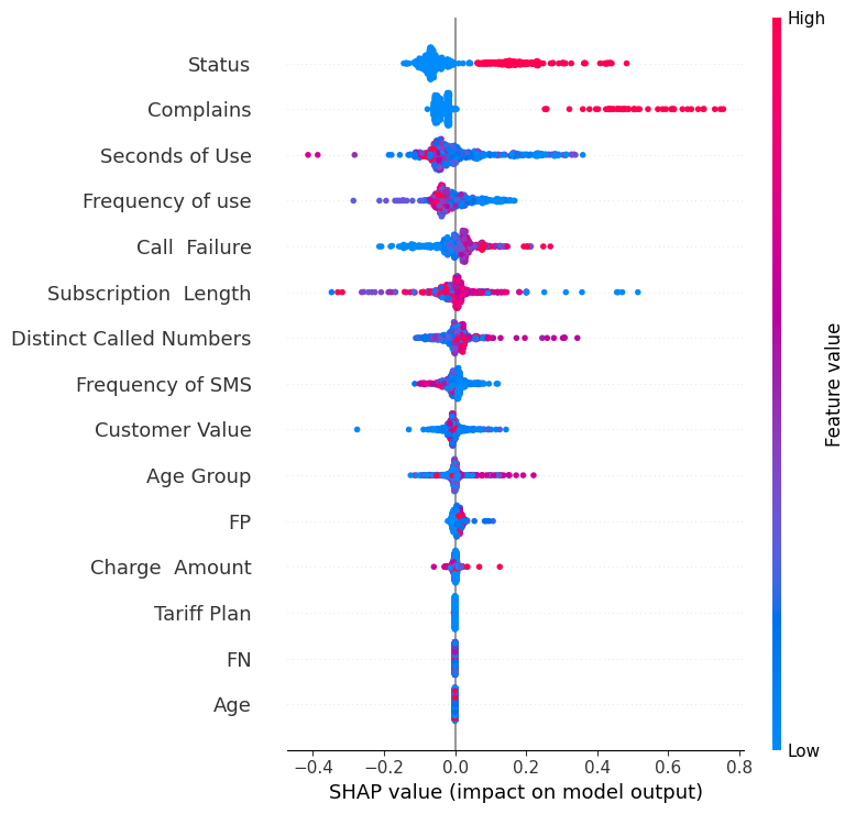
Some additional notes here:

• Y-axis indicates the feature names in order of importance from top to bottom.
• X-axis represents the SHAP value, which indicates the degree of change in log odds.
• The color of each point on the graph represents the value of the corresponding feature, with red indicating high values and blue indicating low values.
• Each point represents a row of data from the original dataset. The gray vertical line in the middle is actually baseline for the prediction. If you look at the “Complains”, which has widest spreading, it tells you that the feature has highest importance and higher value(in our case, 1 over 0) will have largely positive impact on the probability of “churn”.

If you want to look at a local SHAP value, to understand for a single observation, how each figures will add or minus the probability of “churn”, you can do this:

shap.plots.force(explainer.expected_value, shap_values.values[0], X_test.iloc[0], matplotlib = True)

Outputs:

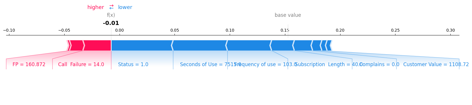
Much straightforward, huh? The baseline is -0.01 and for each feature, the contribution to the final output is quite obvious. The feature FP reduced the chance of ‘churn’ and the feature status increased the chance of ‘churn’ from around -0.01 to 0.05, for example.

Comes here a big ‘BUT’! With the surging popularity of Large Language Model, the dozens of billions of parameters and the black-box layering structure makes it difficult to explain the reasoning from prompts(inputs) to responses(outputs).

For LLM or deep learning networks, the SHAP values apply in a much concise way. After being tokenized and embedded, the input sentences are in the comfortable position to participate into further mathematical computation and finally being inferenced into output embeddings.

Therefore, they get decoded by the same tokenization rule, ending up as the final response from the LLM. These embeddings embodies the probability of each ‘next’ word. And it is the same probability marginal contributions are calculated upon. Let us take a simple example:

#!pip install datasets
#!pip install transformers
#!pip install scipy
#!pip isntall torch
import datasets
import numpy as np
import scipy as sp
import torch
import transformers

# load a BERT sentiment analysis model
tokenizer = transformers.DistilBertTokenizerFast.from_pretrained("distilbert-base-uncased")
model = transformers.DistilBertForSequenceClassification.from_pretrained("distilbert-base-uncased-finetuned-sst-2-english")


# define a prediction function
#any function which will take input data into output response can be seen as prediction function and used in the explainer
def f(x):
    tv = torch.tensor([tokenizer.encode(v, padding="max_length", max_length=500, truncation=True) for v in x])
   # tv=tokenizer(x, padding=True, max_length=200, truncation=True, return_tensors='pt')
    outputs = model(tv).logits.detach()
    #scores = (np.exp(outputs).T / np.exp(outputs).sum(-1)).T
    scores=torch.softmax(outputs,dim=-1)
    val = sp.special.logit(scores[:, 1])  # use one vs rest logit units
    return val


# build an explainer using a token masker
explainer = shap.Explainer(f, tokenizer)

# explain the model's predictions on IMDB reviews
imdb_train = datasets.load_dataset("imdb")["train"]
shap_values = explainer(imdb_train[:10]['text'])

shap.plots.text(shap_values[2])

shap.plots.bar(shap_values.abs.mean(0))

Some additional notes:

• Using tokenizer as token masker for Explainer to automatically mask different words for marginal contributions calculation.
• Masking,in some sense, means changing. It can change the word into another word or hide the word from processing
• If you don’t want to define own prediction function, using model as the first parameter in the Explainer.

What is LIME

LIME (Local Interpretable Model-Agnostic Explanations) is a technique used to explain individual predictions of any black-box model by approximating it with a simpler, interpretable model.

Let’s break this down:

• Local → Focuses on one specific prediction, not the entire model.
• Interpretable → Uses simple models like linear regression or decision trees for explanation.
• Model-Agnostic → Works with any machine learning model (neural networks, random forests, LLMs, etc.).

In plain English, let me put this way:

Any black-box model(Model-Agnostic in this sense) hardly bears any information regarding how the prediction is made, and the LIME will leverage approximation method to retrieve a set of weights(coefficients in linear regression, for example) to clarify on how the prediction is made from individual input(that is what "local" means).

How LIME is calculated

First of all, assume we have a sentiment analysis model that predicts whether a review is Positive (1) or Negative (0). Given this review: "The movie was absolutely fantastic and wonderful."

Assume again that our model f(x) predicts Positive (1) with 90% confidence.

Then LIME normally deployed four steps methods to help explain why prediction go that way.

Step1 Define the prediction function

The prediction function can be a model or just a function, assume we have a model or function f(x), it works this way per our assumption previously mentioned: Review: "The movie was absolutely fantastic and wonderful." Model prediction f(x) : 0.9

Step2 Generate perturbed samples

LIME will randomly marked words and feed them into the model to have a new prediction, as shown below:

Perturbed Samples	Model Prediction $f(x_i’)$
"[MASK] movie was absolutely fantastic and wonderful."	0.85
"The [MASK] was absolutely fantastic and wonderful."	0.60
"The movie was absolutely [MASK] and wonderful."	0.40
"The movie was absolutely fantastic and [MASK]."	0.75

This tell us how much the words contribute to the final prediction(by masking them).

Step3 Assign Similarity Weights

we are actually perturbing the text, and we want to know how far the perturbed text are from the original version so we have knowledge on how much the difference between prediction matters. LIME uses an exponential kernel function:

where:

• $d(x,x_i′)$ is how much the perturbed sample differs from the original.
• $σ$ is a scaling factor (controls decay).

Distance calculations are out of the scope of this article, but chunks of materials are available. We then add the weights into the perturbed sample table as below:

Perturbed Samples	Model Prediction $f(x_i’)$	Weights $\pi(x,x_i)$
"[MASK] movie was absolutely fantastic and wonderful."	0.85	0.95
"The [MASK] was absolutely fantastic and wonderful."	0.60	0.80
"The movie was absolutely [MASK] and wonderful."	0.40	0.60
"The movie was absolutely fantastic and [MASK]."	0.75	0.90

Step 4 Fit a simple interpretable model

We want to solve a model, by making g(x) the approximation to f(x) and find the model that represent the f(x) with slighest variation. To achieve that, in the machine learning world, we will define the loss function indirectly as below:

We define g(x) as a simple linear regression: $g(x)=w_0+w_1x_1+w_2x_2+...+w_nx_n$ where $x_i$ represent each words in the text(”fantastic”, for example).There is not much magic about the interpretable model. It is just a linear regression, waiting dataset for problem solving.

Let me try my best to make the logic easy to understand as it is possible:

• we mask the "fantastic" in the original sentence "The movie was absolutely fantastic and wonderful.".
• Let me make the perturbed sentense "The movie was absolutely [MASK] and wonderful." as $x_1$ and feed into the model f
• Therefore, we now have 0.4 as output from $f(x_1)$ and 0.6 as the computed $\pi(x,x_i)$
• We repeat what we are doing for all single words and get all the $f(x_i)$ and $\pi(x,x_i)$, $i \in N=1,...n$ while n is the number of words in the sentence
• all the values from above visually come together as data set to fit $g(x)$. Visually, they looks like below:

Perturbed Samples	"The"	"movie"	"fantastic"	"wonderful"	$f(x_i’)$	$\pi(x,x_i)$
"[MASK] movie was absolutely fantastic and wonderful."	0	1	1	1	0.85	0.95
"The [MASK] was absolutely fantastic and wonderful."	1	0	1	1	0.60	0.80
"The movie was absolutely [MASK] and wonderful."	1	1	0	1	0.40	0.60
"The movie was absolutely fantastic and [MASK]."	1	1	1	0	0.75	0.90

So the effort we try to solve the weighted least squared problem(solve the loss function) is the same effort we fit the $g(x)$. Just make every word a features, and we can easily:

• fit the $g(x)$ and solve the regression problem
• get Coefficients as w.

We won’t go into mathematical computation for now, and just assume we have finished fitting, and reconstruct the g(x) with textual words as below:

$g(x)=0.35*("fantastic")+0.30*("wonderful")-0.10*("absolutely")+0.05*("movie")+0.15$

Some explanatory notes can be explored:

• Removing "fantastic" reduces confidence by 35%(towards positive prediction)
• Removing "wonderful" reduces confidence by 30%.
• Removing "movie" has little effect (5%).
• The minus w (-0.10) here will add confidence of predicting negative

Let us see the codes below

#!pip install lime
#!pip install transformers
import torch
from transformers import AutoModelForSequenceClassification, AutoTokenizer
import numpy as np
from lime.lime_text import LimeTextExplainer

# Load pre-trained model and tokenizer
model_name = "distilbert-base-uncased-finetuned-sst-2-english"
tokenizer = AutoTokenizer.from_pretrained(model_name)
model = AutoModelForSequenceClassification.from_pretrained(model_name)

# Function to predict sentiment probabilities
def predict_proba(texts):
    inputs = tokenizer(texts, padding=True, truncation=True, return_tensors="pt")
    with torch.no_grad():
        outputs = model(**inputs).logits
        probabilities = torch.nn.functional.softmax(outputs, dim=1).numpy()
    return probabilities

# Create a LIME explainer
explainer = LimeTextExplainer(class_names=["Negative", "Positive"])

# Example sentence for explanation
text = "I absolutely loved the movie! But the supporting actors are not good."

# Generate LIME explanation
exp = explainer.explain_instance(text, predict_proba, num_features=10)

# Show explanation in Jupyter Notebook
exp.show_in_notebook(text=True)

Output might be something like below:

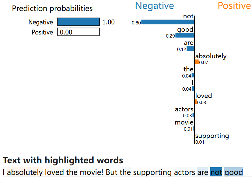
Additional notes:

• We download tokenizer and model from huggingface for sensitivity analysis
• Define your own function to better control the sensitivity output logic
• On barchart, each words contributing to +/- prediction were listed by importance on left or right side, with darkblue denoting negative prediction and organge denoting the positive one
• Beside barchart, the text in the whole sentence is also colored respectively

Conclusion

Challenges in Explanability

Despite its importance, making AI models explainable isn’t always straightforward. Some key challenges include:

• Complexity vs. Interpretability: More complex models often perform better but are harder to explain or resources consuming
• Scalability Issues: Explanability techniques can be computationally expensive and difficult to apply in real-time.
• Different Needs for Different Stakeholders: A data scientist, regulator, and end-user may all require different levels of explanation.
• Security Risks: Too much transparency can make AI systems vulnerable to adversarial attacks or exploitation. It is raising attack alarm therefore.

Evolution in Explanability in AI

As AI continues to evolve, so too will our ability to make it more explainable. Future advancements may include:

• Self-Explaining AI Models: AI systems that naturally provide justifications for their decisions.
• Hybrid Approaches: Combining multiple explanability techniques for greater clarity.
• Industry Standards: Establishing guidelines for how AI models should be evaluated for transparency and fairness.

As human beging, we just wish the surging popularity of AI(ML, LLM, etc) are doing their job for the better of us, not harm to us. It is critical that we understand why they do, act or response in this way before they do something that does not make sense. Remember: By AI, For Human.

---

Author: Jun Ma, co-founder of obserpedia